Model
Lithospheric Magnetization Model 1 (LMM1)
A global 1°×1° model of lithospheric magnetization strength derived from petrologic and satellite data inversion.
Model Overview
This model presents the global distribution of lithospheric induced magnetization, expressed as Vertical Integrated Susceptibility (VIS). It is derived from a joint inversion of satellite magnetic observations (CHAOS-8) and petrological constraints (SM3-SI) using a spherical equivalent source layer, with a spatial resolution of approximately 1°. The model covers spherical harmonic degrees 0–80, including the long-wavelength components of the lithospheric field that are normally masked by the core field. It clearly resolves magnetization contrasts across different crustal types and tectonic settings, and is well suited for studying magnetic structures of Precambrian cratons, orogenic belts, subduction zones, and oceanic plateaus.
Model Visualization
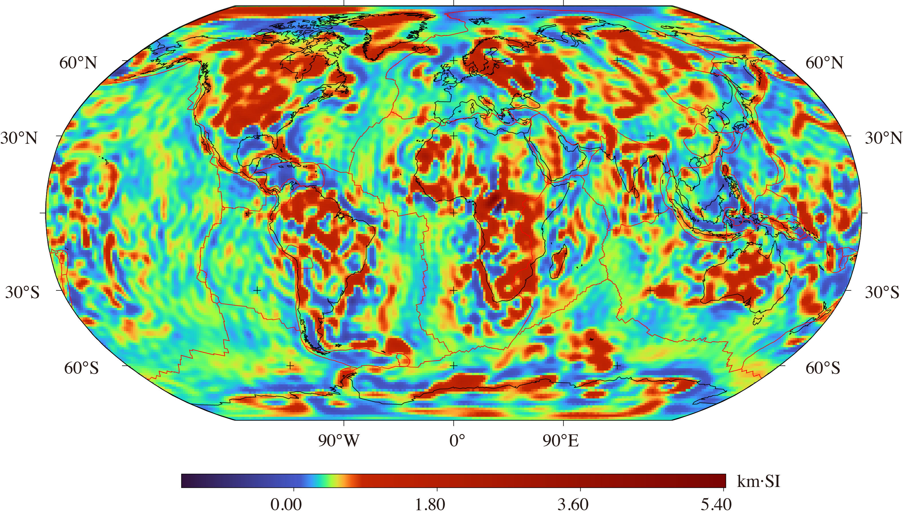
Inverted VIS model of the lithospheric induced magnetization. Continental and plate boundaries are drawn in black and red lines, respectively.
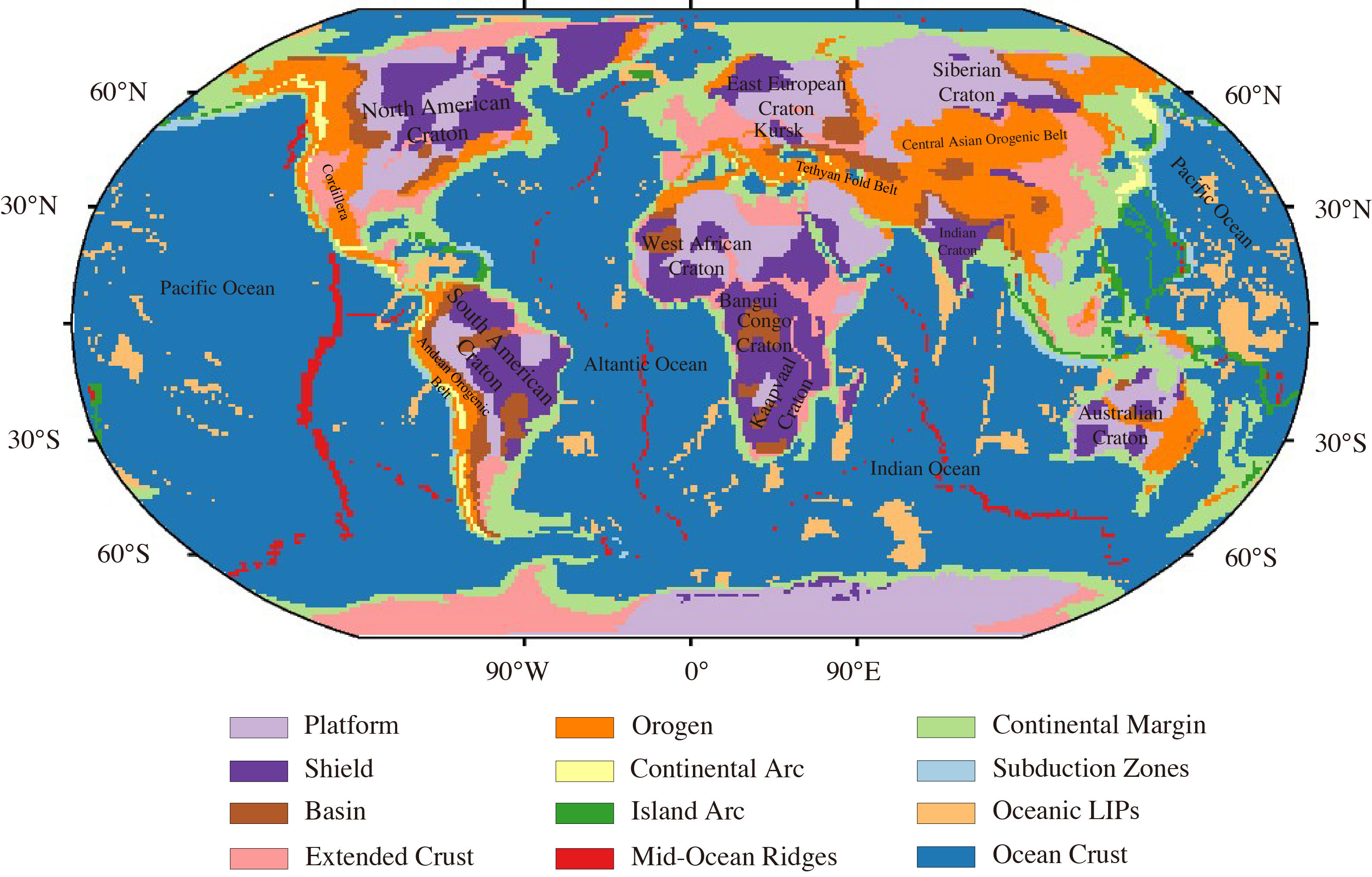
Global crustal-type map (Mooney et al., 2023), which shows twelve crustal units. Major tectonic regions are labeled. A MapGIS version of this map could be found at ECM1.
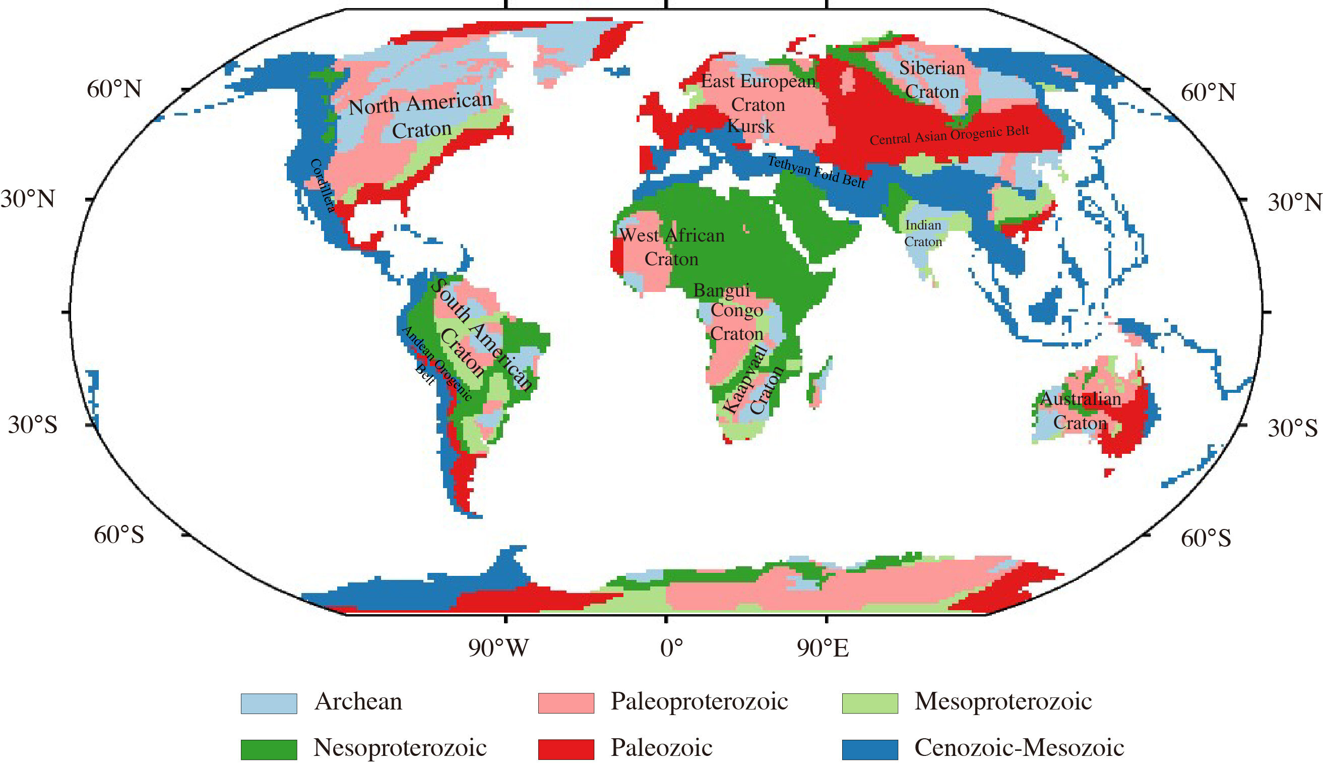
Continental basement age map (Gubanov & Mooney, 2009, 2014; Mooney et al., 2025), which shows six age units: Achaean (3.8–2.5 Ga), Paleoproterozoic (2.5–1.6 Ga), Mesoproterozoic (1.6–1.0 Ga), Neoproterozoic (1.0–0.54 Ga), Paleozoic (543–250 Ma), and Mesozoic-Cenozoic (250–0 Ma). Major tectonic regions are labeled. A MapGIS version of this map could be found at ECM1.
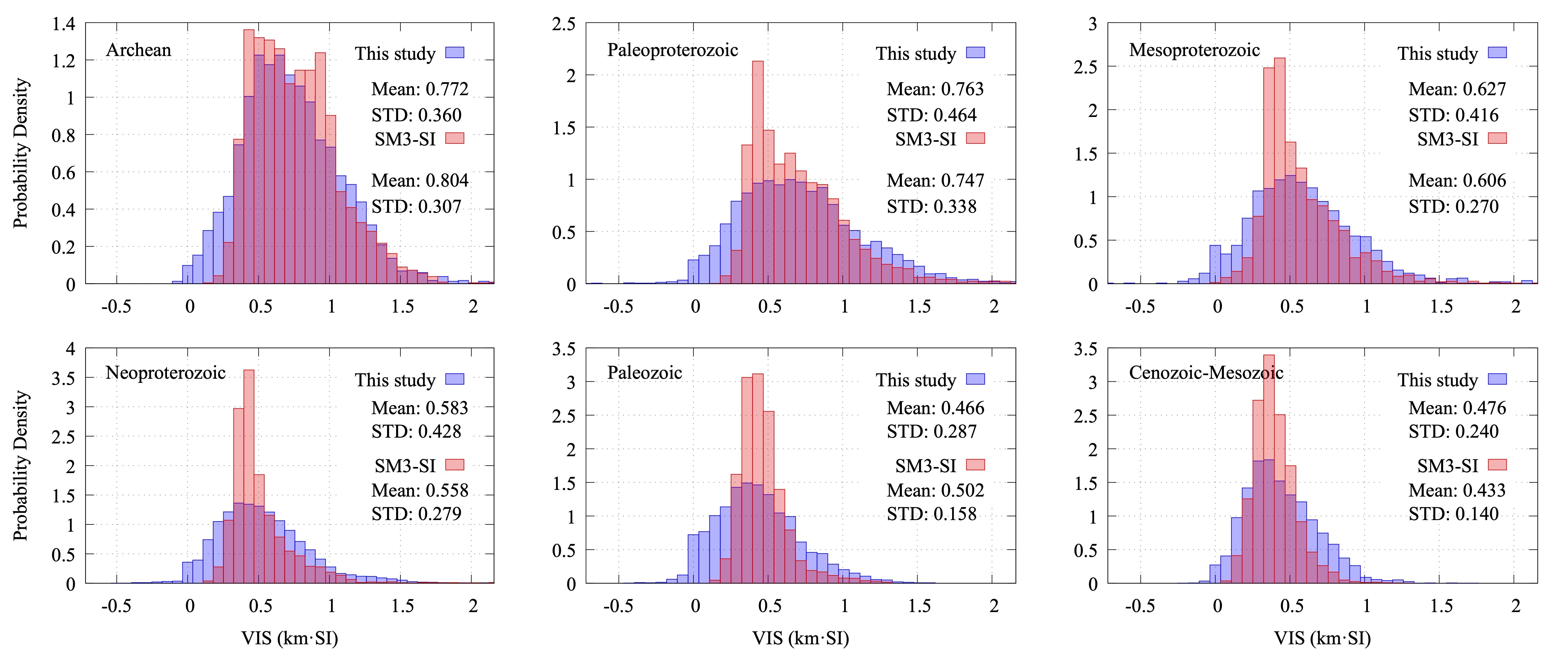
Histograms of the inverted VIS model of the lithospheric induced magnetization grouped by different basement ages. Statistics from the SM3-SI model (Hemant & Maus, 2005) are also shown for comparison.
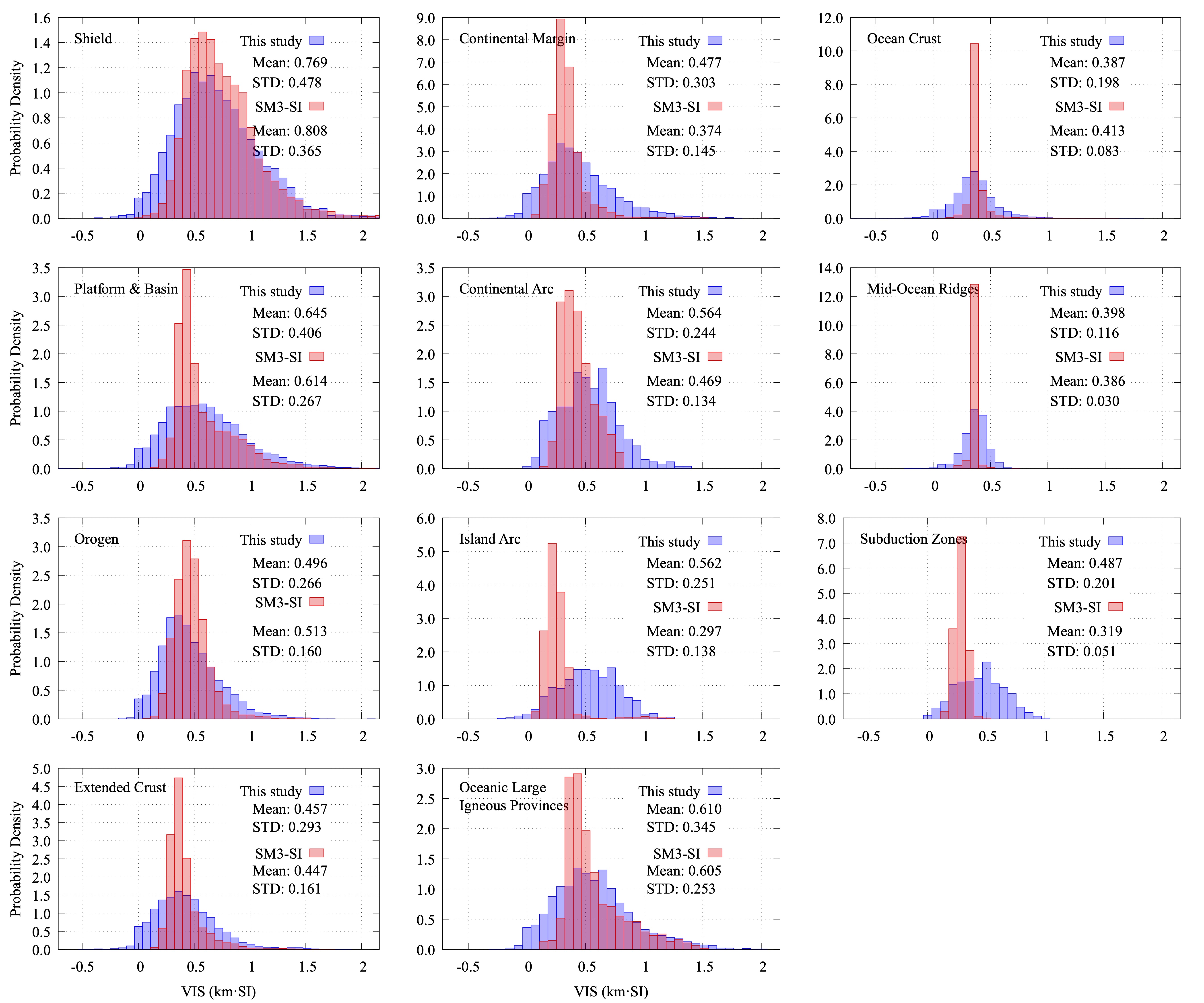
Histograms of the inverted VIS model of the lithospheric induced magnetization grouped by different crustal types. Statistics from the SM3-SI model (Hemant & Maus, 2005) are also shown for comparison.
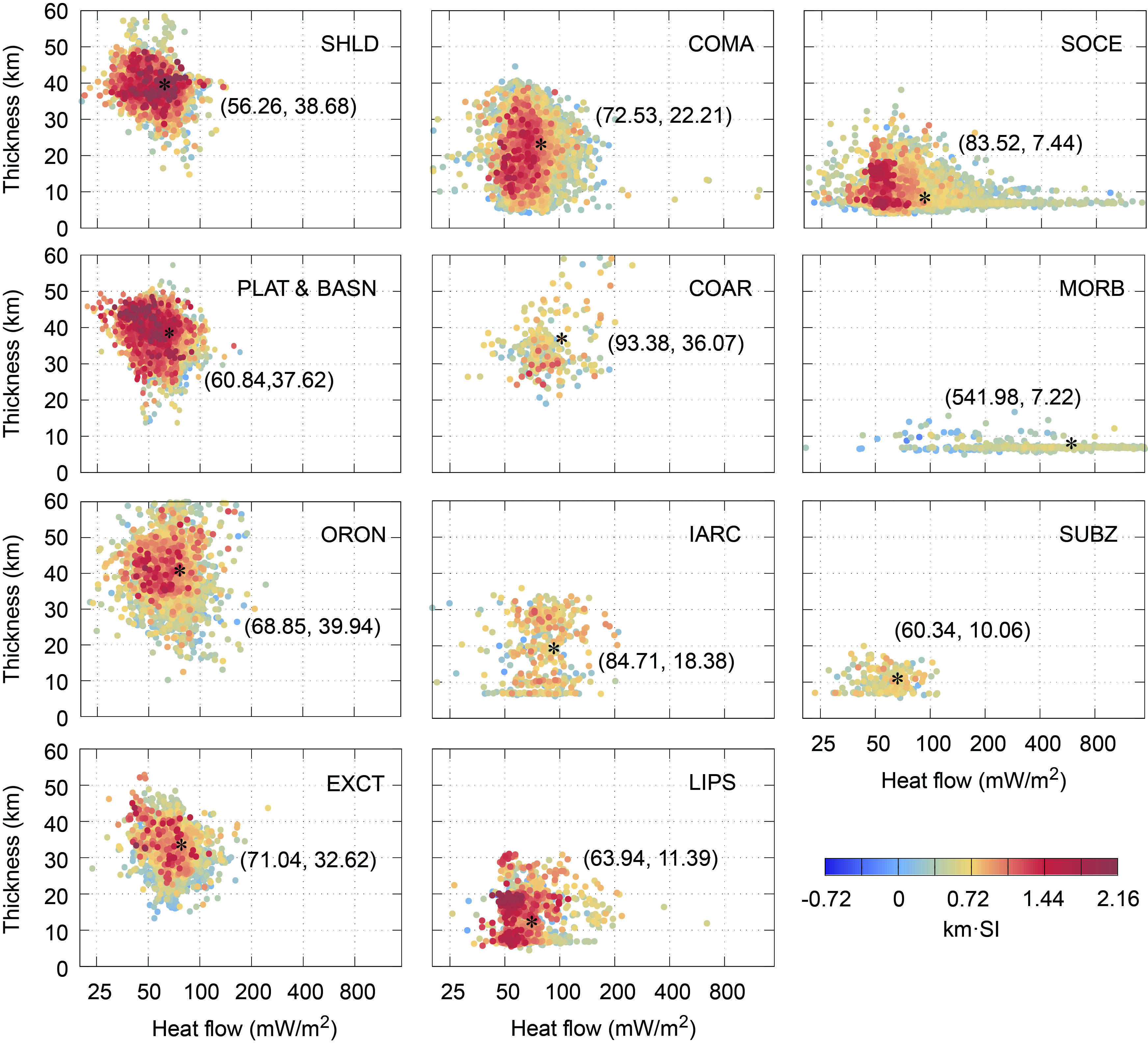
Scatter plots of the inverted VIS values versus the predicted global heat flows (Lucazeau, 2019) and crystalline crust thickness from the ECM1 model (Mooney et al., 2023). The VIS values are grouped by different crustal types (Figure 2). Cluster centers are marked as black stars, with their coordinate positions shown in the figure. To match heat flow and crustal data, the VIS model is interpolated onto a global uniform grid of 1‐degree resolution.
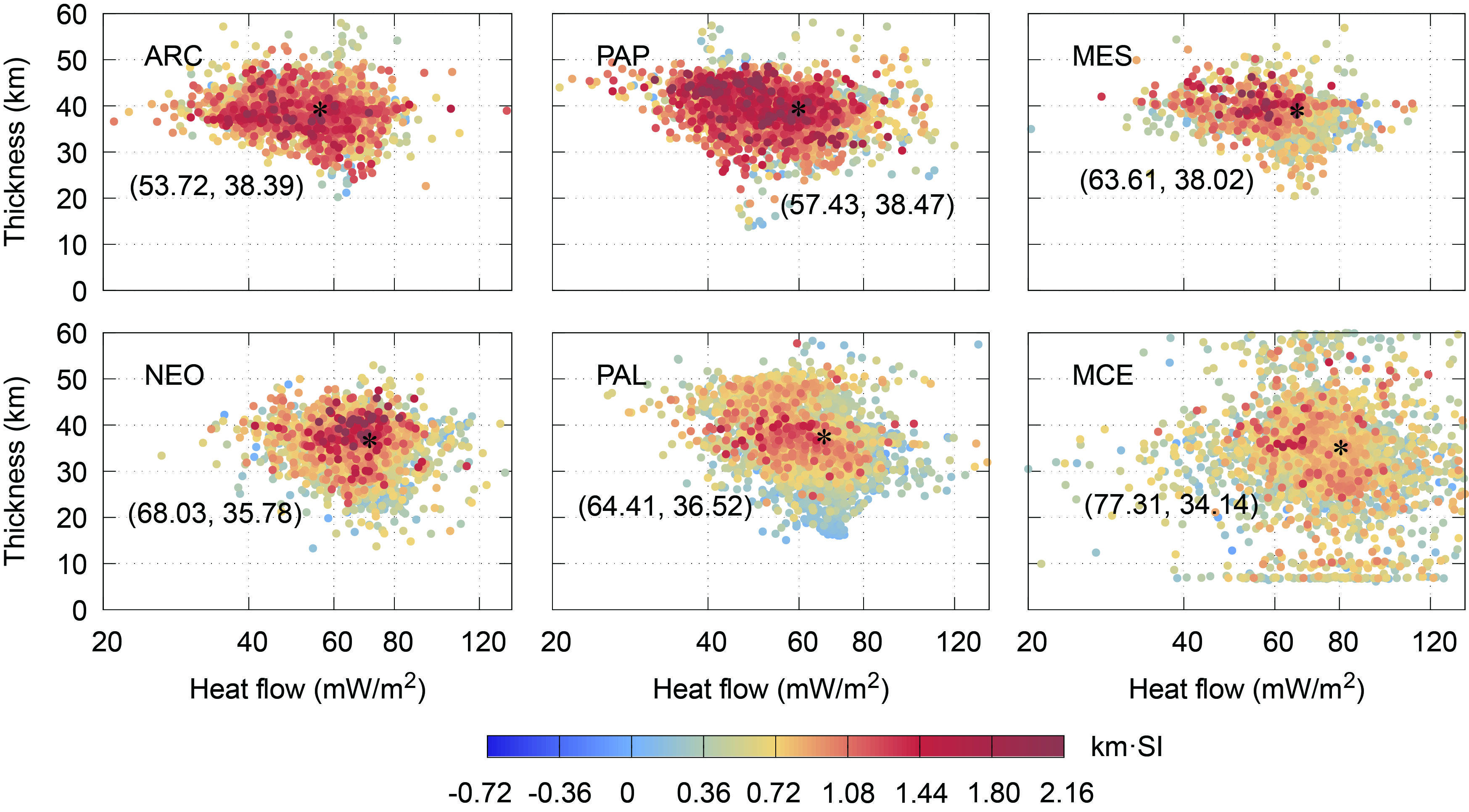
Scatter plots of the inverted VIS values versus the predicted global heat flows (Lucazeau, 2019) and crystalline crust thickness from the ECM1 model (Mooney et al., 2023). The VIS values are grouped by different age units (Figure 3). Cluster centers are marked as black stars, with their coordinate positions shown in the figure. To match heat flow and crustal data, the VIS model is interpolated onto a global uniform grid of 1‐degree resolution.
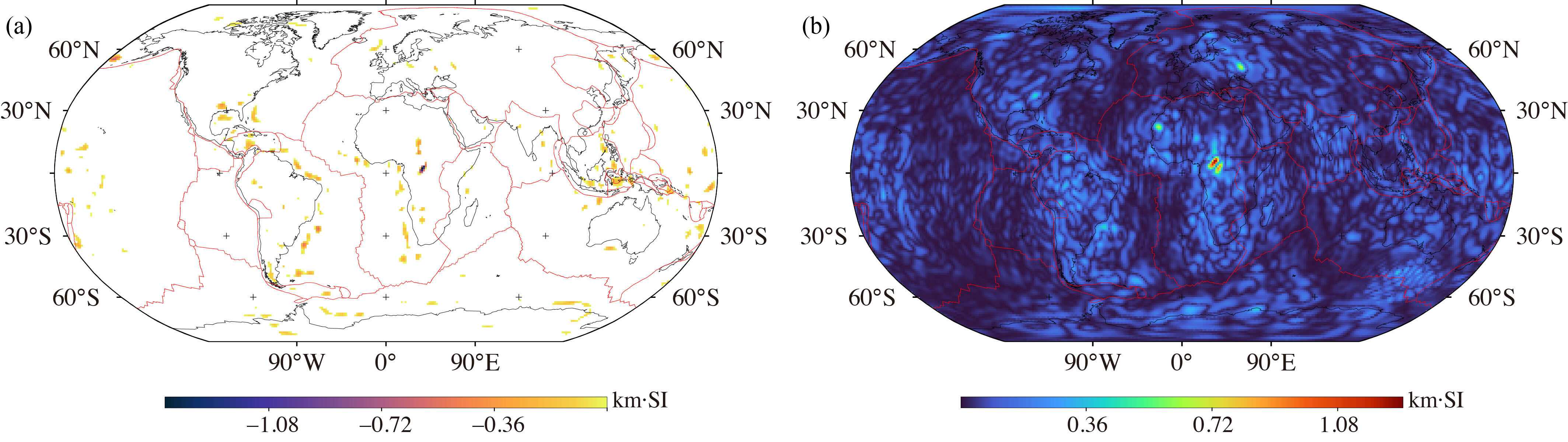
(a) Distribution of the negative values and (b) estimated uncertainties of the inverted VIS model of the lithospheric induced magnetization using constraints from the SM3-SI model (Hemant & Maus, 2005) and CHAOS-8 satellite data (Kloss et al., 2024).
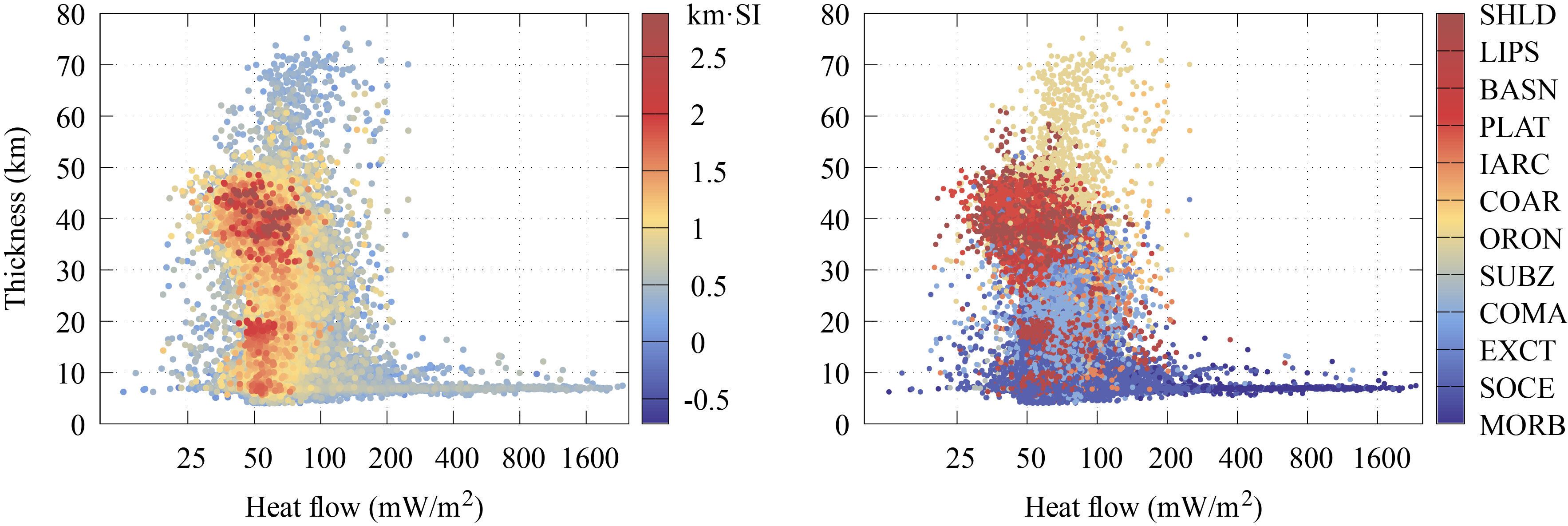
(a) Scatter plots of the inverted VIS values versus the predicted global heat flows (Lucazeau, 2019) and crystalline crust thickness from the ECM1 model (Mooney et al., 2023). (b) Crustal‐type scatter plot, with colors denoting the crustal type for each point shown in (a). To match heat flow and crustal data, the VIS model is interpolated onto a global uniform grid of 1‐degree resolution.
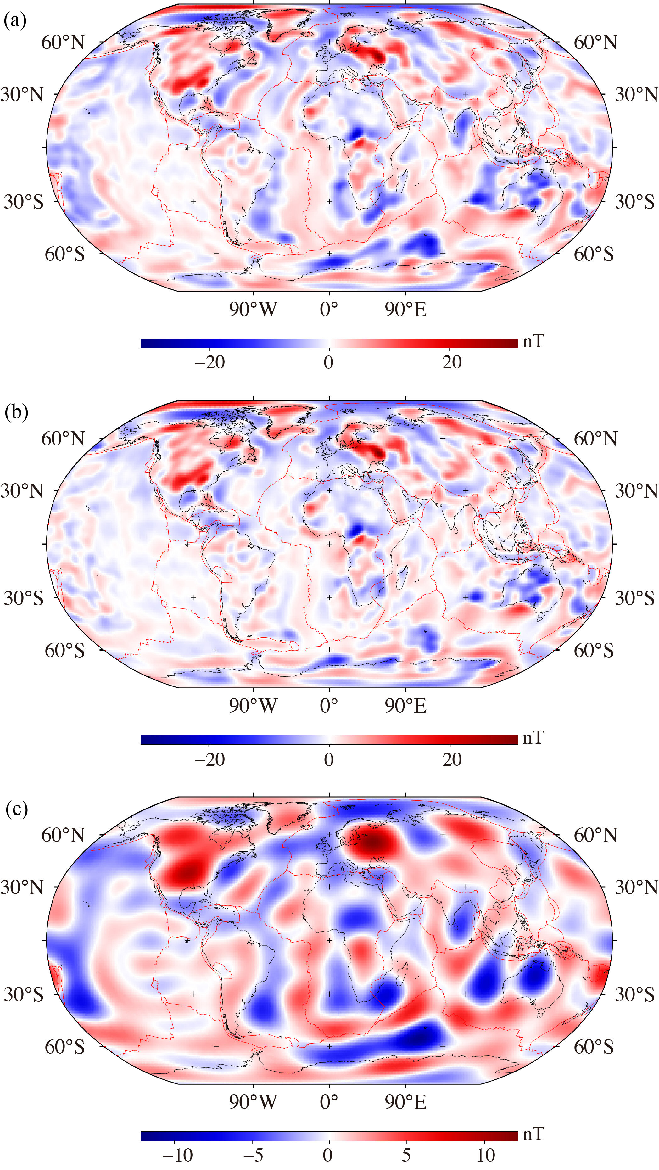
(a) Reproduced Br component of the lithosphere including the remanent magnetic field, (b) reproduced induced Br component of the lithosphere, and (c) reproduced long‐wavelength Br anomalies (SH degrees 1–15). The magnetic data are calculated at a 400 km altitude.
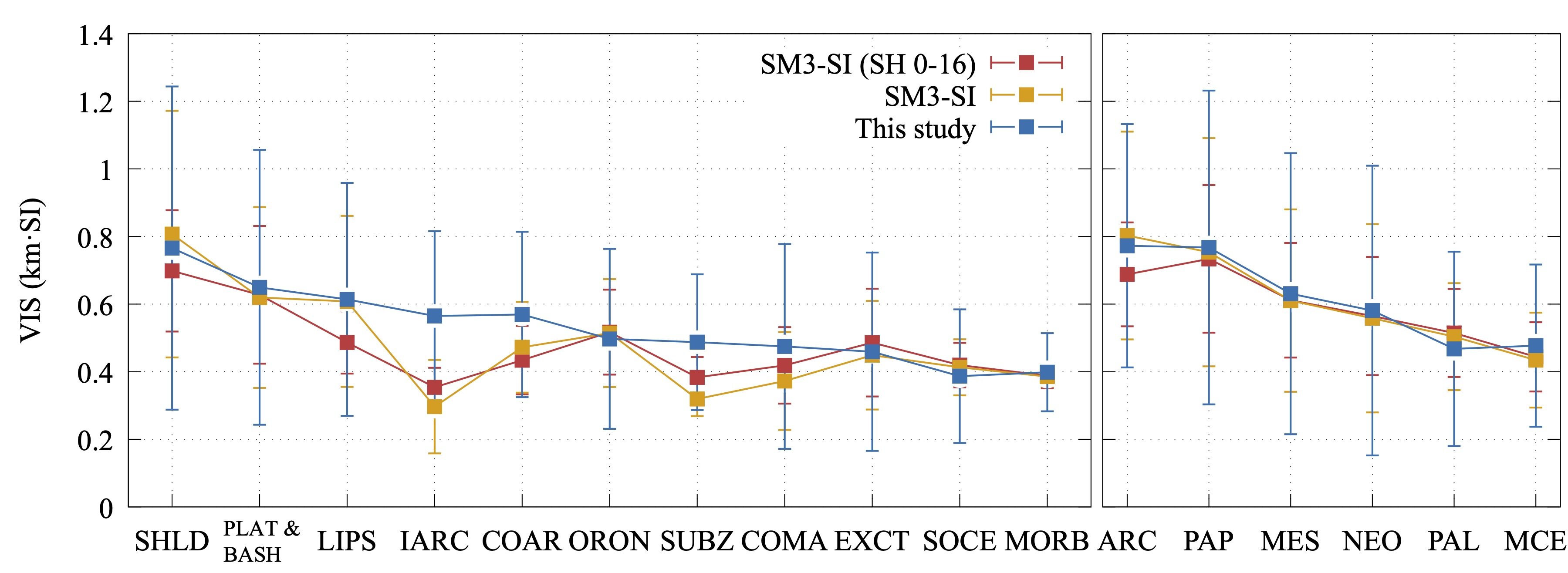
Comparison of area‐weighted mean VIS values between the inverted model and the SM3‐SI model (including its long‐wavelength component from Hemant & Maus, 2005) across different crustal types (left panel) and basement ages (right panel). Corresponding statistics are presented in corresponding paper. Vertical short lines indicate ±1 standard deviations. Spatial regions of the groups are shown in Figures 2 and 3. Histograms and statistics of the groups are shown in Figures 4 and 5, respectively. SHLD, Shield; PLAT, Platform; BASN, Basin; ORON, Orogen; EXCT, Extended Crust; COMA, Continental Margin; COAR, Continental Arc; IARC, Island Arc; LIPS, Oceanic Large Igneous Provinces (LIPs); SOCE, Ocean Crust; MORB, MidOcean Ridges; SUBZ, Subduction Zones; ARC, Archean; PAP, Paleoproterozoic; MES, Mesoproterozoic; NEO, Neoproterozoic. PAL, Paleozoic; MCE, Mesozoic‐Cenozoic.
Data Downloads
All files are released for academic research and teaching. Please read the README before use and cite the model in your publications.
LMM1.csv
Global susceptibility model on a spherical triangular grid, directly output by the inversion program. To obtain the Vertical Integrated Susceptibility (VIS), multiply by the 36 km equivalent layer thickness.
LMM1_mag_shc.csv
Spherical harmonic coefficients of the lithospheric magnetic field model corresponding to the inverted susceptibility model, allowing users to compute the lithospheric magnetic field at any desired spherical harmonic degree.
LMM1_sus_grid.csv
Gridded global susceptibility model at 1° × 1° resolution.
LMM1_sus_grid.nc
Gridded global susceptibility model at 1° × 1° resolution (netCDF format).
Zhang, Y., Sun, S., Mooney, W. D., & Xu, Y. (2026). Lithospheric Magnetization Derived From Petrological and Satellite Constraints. Journal of Geophysical Research: Solid Earth, 131(1), e2025JB032111. https://doi.org/10.1029/2025JB032111